Motion Kinematics

In this white paper, we look at machines with non-Cartesian movement systems. These include nearly all 'armed' robots such as SCARA (Selective Compliant Assembly Robot Arm) robots, PUMA (Programmable Universal Manipulation Arm)-style arms, Delta Robots, as well as various other mechanisms.

These non-Cartesian mechanisms are often still required to operate in a Cartesian workspace. This presents special challenges, but there are some basic techniques that will take you a long way toward getting these useful and common mechanisms under control. So, let’s get started!

My M.E. built a robot arm and all I got was this stupid non-cartesian control challenge

There are broad classes of machines that use a Cartesian mechanism to translate movement from one desired position to another. A simple example is an X-Y table. Each motor directly drives the load in either the X direction or the Y direction. When a third direction (Z) is added, the device is commonly referred to as a gantry.

Complex objects such as lines and ovals are accomplished by coordinating the motion of each axis so that the desired multi-dimensional object is created. Figure 1 shows a Cartesian motion system in the process of drawing a circle.

When the motion system is Cartesian, drawing objects that are expressed as a Cartesian algebraic equation (y=f(x)) may not be straightforward. By definition, for any value of the independent variable (x), the dependent variable (y) can only have one value, which eliminates a large number of conceivable XY paths. You may recognize the equations for a circle, given below:

Motion Kinematics
(eq. 1)

Motion Kinematics
(eq. 2)

fig-cartesian-motion-system-pmdcorp
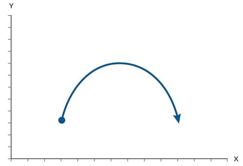
Figure 1: Cartesian motion system

We're not in Cartesia anymore

But what if the motion mechanism is not based on a simple X and Y (Cartesian) mechanism? In that case, just translating actuator motion (typically rotary motors) to real-world coordinates such as X and Y is a chore, and performing straight line moves or circles is even more challenging.

Figure 2 shows an assembly robot arm known as a SCARA arm. In the most common SCARA robot configuration, there are four axes of motion, although only two, the shoulder rotary motion and the elbow rotary motion contribute to the destination location of the load point in the XY plane. The third axis is the wrist, which is a spinning motor at the end effector, and the fourth axis moves the entire arm up and down.

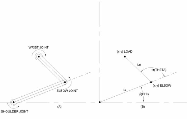
Figure 2: SCARA robot arm and coordinate system

How do the two main motion actuators, the shoulder joint and the elbow joint, create motion at the end effector? To answer this, we will calculate what is known as the forward kinematics of a SCARA arm. That is, equations which translate the shoulder and elbow actuator motion into X and Y coordinates of the end effector.

The equations, which denote the shoulder-connected segment as length Ls, the elbow-connected segment as Length Le, the shoulder angle as Phi (ϕ), and the elbow angle as Theta (θ), are given below:

SCARA robot arm and coordinate system
(eq. 3)

Motion Kinematics
(eq. 4)

So far, so good. If we know the shoulder and arm angle, we can now calculate what the X and Y axis coordinates of the end effector are.

We are living in a Cartesian world

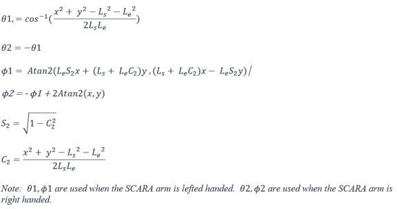
The SCARA is still required to operate in a cartesian workspace which means controlling the XY position of the end effector. The shoulder and elbow angles must be calculated for a given X and Y end effector location. This is called inverse kinematics, and for SCARA arms and many other non-Cartesian motion systems, this is more complicated to calculate then forward kinematics.

To begin with, there are two ways to get to every location in the motion plane. Think of your own shoulder and elbow, and imagine reaching for an object left handed, and then right handed. Either arm can arrive at the same location, mirror images of each other. A human elbow cannot exceed a 'straight elbow' angle, but a single SCARA arm has no such constraint, so it can move to the object in either manner; left handed or right handed.

Nevertheless, using the law of cosines and basic trigonometry we can come up with the equations for the shoulder angle (Phi) and the elbow angle (Theta) given X and Y. Again, without derivation, here they are:

equation-motion-kinematics-pmdcorp

Start your engines! And then turn them off

With this trigonometric head bender behind us, we are ready for action, right? Hardly. In fact, we're just getting started.

Let's take a simple example. Assume we want to move the SCARA arm from one XY location to another in a straight line. This is shown in Figure 3, where a move from XY location (8, 4) to location (-4, 8) has been diagrammed.

Motion Kinematics
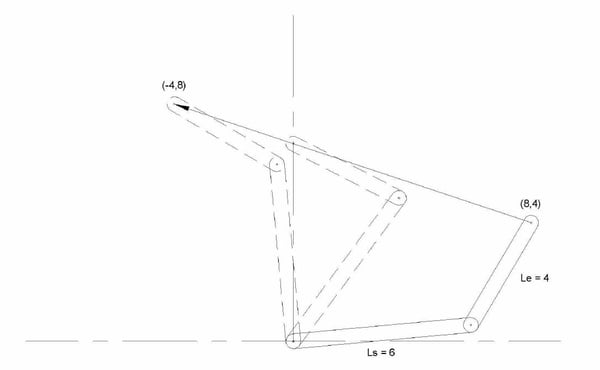
Figure 3: SCARA arm – move from (8, 4) to (-4, 8)

If we use the inverse motion kinematic equations from above to determine the starting shoulder and elbow positions, and command a simple move to travel to the shoulder and elbow destinations, we will find that the path traveled is not straight in the X-Y plane.

Why is this? The reason becomes clear if we plot the points on the desired straight line path and look at the corresponding graph of Phi and Theta. This is shown in Figure 4a.

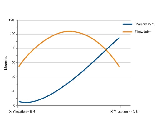SCARA Arm Movement Figure 4a: Shoulder and Elbow angles during straight line move from (8, 4) to (-4, +8)

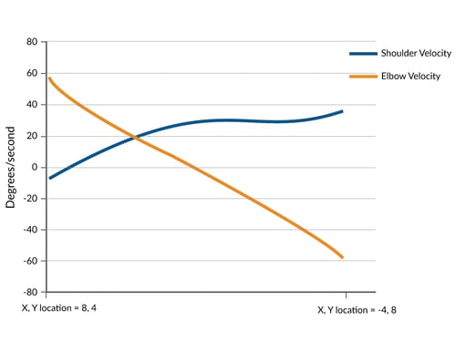SCARA Arm Velocity Control Figure 4b: Shoulder and Elbow velocity during straight line move from (8, 4) to (-4, +8)

Due to the non-Cartesian mechanical linkage, the motors rotate much faster at some points and much slower at other points to keep the load on a straight line path. The resultant profile is complex, resembling neither a trapezoid nor other standard off-the-shelf trajectory forms.

Some applications may not care if the load does not travel in a straight line, but most will. If the system response is dominated by the load and the path is not a straight line extra energy will be expended and servo tracking will be more difficult due to unwanted side-to-side movement of the load.

This is the primary challenge of controlling non-Cartesian mechanisms; to continuously tailor the commanded position in the robot's non-Cartesian motor actuator space such that the inverse kinematic equations are adhered to.

Since we have the equations, the easy part is knowing what we want to do in the XY space. The tricky part is designing a control system that can elegantly (ideally invisibly) translate these XY trajectories into the continuously contoured actuator paths that adhere to the inverse kinematic space of the mechanism.

A new trajectory

Fortunately, there are a few approaches you can use. To begin with, it is possible that your motion controller allows you to download math equations using software code and has the computing power to perform inverse kinematics on-the-fly.

If you choose this approach, you will take the output of the motion controller's standard X-Y space profile generator and run it through the inverse kinematic equations. These equations need to be programmed directly into the controller's motion engine using the vendor's programming language. Unfortunately, both this capability, and this level of compute power for equations as complex as eq (3), is rare in off-the-shelf motion controllers.

Another approach, and perhaps the most common method used until relatively recently, is to break the profile into pieces and use segments of a standard profiling capability, such as a trapezoid, to execute a complex shaped path. Even just a few segments will dramatically improve the accuracy of the kinematic track. If you break the move into dozens or hundreds of pieces, using this approach can give very acceptable results for most machines.

The main downside of this segmented profile approach is that it requires a lot of work from the supervisor software program. You must continuously monitor where the profile is, and feed in the next segment at the right time.

This is made easier using position comparison breakpoints, so at a minimum confirm that your motion controller supports pre-storage (also called buffering) of profile breakpoints to allow segments to be fed in automatically.

All of this aside, segmentation of the profile can work, but it is awkward to implement and has significant limitations. On-the-fly changes of the profile are pretty much out of the question, because segment tables are generally pre-generated. And if you attempt to make point to point moves with higher order velocity contours such as S-curves, the complexity ratchets up quickly, and segmentation becomes proportionally more difficult.

You may also be interested in: S-Curve Motion Profiles - Vital For Optimizing Machine Performance

You're my only hope, O' translation table

This brings us to a third approach, one that neatly solves a number of these problems. The general technique uses translation lookup tables to perform reference frame conversions on-the-fly. Here is how it works.

From the data in Figure 4a, we see that each X or Y point maps to a specific Phi and Theta point. If we put these point pairs into a lookup table, we have a system that can execute a standard profile in XY space and then automatically convert this, using the translation lookup table, into the appropriate Phi Theta space for output to the actuators.

Translation tables used in this way are very close cousins to the profiling technique called camming (electronic cam). In camming, the input reference is an encoder position, and the output is the motor actuator command. Each encoder input position has a unique mapping to the output command, allowing arbitrary shapes to be executed automatically and repeatedly.

Translation tables make an effective inverse-kinematic engine. First and foremost, translation tables reduce the need for real time computation since the supervisory computer takes as much time as it needs to pre-calculate and download the inverse kinematic curves. Execution of the profile by the motion controller happens in real time, via a simple and fast lookup operation.

Beyond that, when translation tables are used with a cam-like lookup mechanism they allow us to separate the profile path from the velocity with which that path is traversed. In a moment we will show how this provides a very powerful and flexible approach to control the velocity of complex, kinematically accurate moves.

Some practical notes: Although the cost of digital memory is quite low, translation tables for every possible input point are impractical. Typical systems utilize spline segments, either 2nd order or 3rd order, to interpolate between lookup values. This lowers the total number of points that need to be pre-calculated and downloaded.

In the example of the SCARA arm where we want to convert XY commands to Phi, Theta commands, what we want is a two-dimensional translation table. But a two-dimensional cam-style table would take up large amounts of memory.

The solution is to create tables, not for all possible moves, but only for the specific library of moves that are needed. Most motion systems utilize only a limited repertoire of moves, such as "extend straight out", "retract straight in", or "move from station #3 to station #8", etc.

Putting it all together

By now your head is probably spinning, so let's come back down to earth by giving a real example. Let's go back to the SCARA arm move earlier in the deep dive and show how we would use cam-like lookup tables to draw the straight line from that example.

We want to make a move from (8, 4) to (-4, 8) so we break the move into a number of cam segments (the more segments, the more accurate the tracking, although generally for simple objects 50 segments is plenty). One cam table will hold all the Phi (shoulder) actuator values, and another will hold all the Theta (elbow) actuator values.

Phi CAM Table
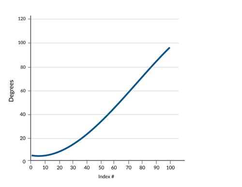
Figure 5a: Phi (shoulder joint) CAM table

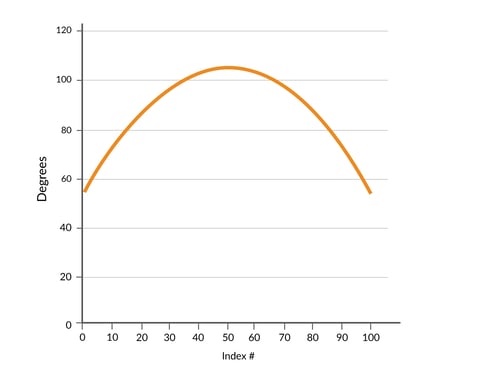Theta CAM Table Figure 5b: Theta (elbow joint) CAM table

This is shown in Figures 5a and 5b. We generate 100 XY points comprising a straight line with equidistant points from the start location to the end location. We then run each of these XY points through the inverse kinematic equations (eq. 6 and 7), to generate the corresponding Phi and Theta points for each index value 1 through 100, and we load them into translation tables, one for the Phi axis and one for the Theta axis.

Now we apply a neat trick. Instead of running a traditional cam profile with the input encoder positions coming from an external encoder source, we 'point' the incoming position data stream to an internal profiled axis of the motion controller. This 'velocity regulator' axis' output, shown in Figure 5c, will be used strictly as input to the Phi and Theta translation tables, taking the place of the normal cam input from an external encoder.

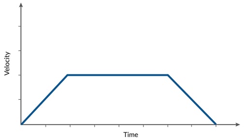
Translation Input for Velocity Reference
Figure 5c: Translation table command input velocity reference

By loading this third velocity regulator axis with trapezoidal or s-curve velocity profiles, we will regulate the speed of the complex Phi, Theta SCARA arm path. We can even stop, reverse directions, or change the velocity on-the-fly if we want. Whatever position data stream is output by this velocity regulator axis, will become the index used for the Phi and Theta translation tables. And they will faithfully track the input position, staying in the correct kinematic relationship to each other.

Voila! We now have a general-purpose technique to control even very complex non-Cartesian mechanisms.

Exercises left for the reader

As useful and convenient as this is, there are limitations.

Probably the main one is that with one-dimensional cam tables such as described above, you must create a separate table for each drawn object. If there are, in fact, no pre-drawn shapes or moves, then this technique will not work.

Another area that is not addressed by the translation table technique is feedfoward. Machine designers always seek maximum performance from their systems, and as I have discussed in past deep dives feedforward is a major tool in this arsenal.

Feedforward typically uses the acceleration profile command to generate an on-the-fly torque compensation value to offset forces resulting from load inertia. As the load accelerates, it injects a boost to fight the tendency of the load to stay at rest, and as the load decelerates, it injects a brake to fight the tendency of the load to stay in motion.

Unfortunately, we cannot feed X or Y-frame feedforward information directly to the Phi or Theta actuators. This is because these forces are subject to the same rules of kinematic conversion as the path profiling is. Worse, the actual reflected torque at the actuator includes entirely new forces such as centripetal force owing to the rotary motion of the shoulder and elbow arms.

So, we will leave torque feedforward for non-Cartesian mechanics as an exercise to the reader. There certainly are methods, such as the Lagrange-Euler (L-E) method, to construct a dynamical model of your system and solve these problems, but for the purposes of this article, we are going to quit while we're ahead!

You may also be interested in: Feedforward in Motion Control - Vital for Improving Position Accuracy

Summary

Many motion control systems contain mechanics that form a non-Cartesian reference frame. These range from simple rotary axes such as a lever interacting with a linear conveyer belt to more complex machines such as SCARA robots, Delta Robots, and more.

The fundamental mathematics of control for these systems are described by forward and inverse kinematics, however these equations can be complex, and create challenges for managing path execution in the inverse-kinematic reference frame.

There are a few techniques to manage this complexity, but translation tables for individual moves that convert the XY reference frame to the non-Cartesian actuator reference frame are an excellent general-purpose approach that allows complex velocity shaping while managing real-time computational needs.

Before we close, below is a video that shows a robot in action with profiles, kinematics, and feedforward all optimized and finely tuned. This type of robot is called a Delta Robot and represents an actuator configuration that has found increasing use in industrial applications, particularly high-speed pick and place applications.

Hope you enjoyed this article, so long till next time.

View video >>

PMD Products Frequently Used In Motion Kinematics Projects

PMD has been producing ICs that provide advanced motion control of DC Brush and Brushless DC motors for more than twenty-five years. Since that time, we have also embedded these ICs into plug and play modules and boards. While different in packaging, all PMD products are controlled by C-Motion, our easy to use motion control language and are ideal for use in medical, laboratory, semiconductor, robotic, and industrial motion control applications.

ION/CME N-Series Digital Drives

N-Series ION Digital Drives combine a single axis Magellan IC and a high performance digital amplifier into an ultra-compact PCB-mountable package. In addition to advanced servo and step motor control, N-Series IONs provide S-curve point to point profiling, field oriented control, downloadable user code, general purpose digital and analog I/O, and much more. With these all-in-one devices building a custom controller board is a snap, requiring you to create just a simple 2 or 4-layer interconnect board.

Learn more >>

Prodigy/CME Machine-Controller

Prodigy®/CME Machine-Controller boards provide high-performance motion control for medical, scientific, automation, industrial, and robotic applications. Available in 1, 2, 3, and 4-axis configurations, these boards support DC brush, Brushless DC, and step motors and allow user-written C-language code to be downloaded and run directly on the board. The Prodigy/CME Machine-Controller has on-board Atlas amplifiers that eliminate the need for external amplifiers. To build a fully functioning system only a single HV power supply, motors, and cabling are needed. Host interface options include Ethernet UDP and TCP, CANbus, RS-232, and RS-485.