
Motion control engineers spend hours optimizing tuning parameters for their servo-based motion controllers. But what if they are using stepper motor controllers? And what if, no matter how much time they spend on tuning, they can’t get the performance they want?
The answer, for many motor control systems, is to focus on the motion profile instead. Advanced profiling features such as asymmetric acceleration and deceleration, 7-segment S-curve profiling, change-on-the-fly, and electronic camming are now widely available, providing engineers with new tools that make machines work faster and more efficiently. This article will take you through the mathematics of motion profiles and discuss which profiles work best for which applications. It will also provide insights into how to “tune” your motion profile for maximum performance.
S-Curve and Trapezoidal Motion Profiles
While there are a lot of different motion profiles in use today, a good starting point is the point-to-point move. For a large number of applications including medical automation, scientific instrumentation, pointing systems, and many types of general automation, the point-to-point move is used more frequently than any other motion control profile. Because of this, optimization of this profile will have the largest overall impact on system performance. Point-to-point means that from a stop, the load is accelerated to a constant velocity, and then decelerated such that the final acceleration, and velocity, are zero at the moment the load arrives at the programmed destination.
The two profiles commonly used for point-to-point profiling are the S-curve profile, and its simpler cousin the trapezoidal profile. They are shown in Figure 1.
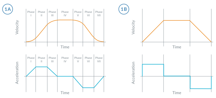
Figure 1: S-Curve Profile and Trapezoidal Profile
In the context of a point-to-point move, a full S-curve motion profile consists of 7 distinct phases of motion. Phase I starts moving the load from rest at a linearly increasing acceleration until it reaches the maximum acceleration. In Phase II, the profile accelerates at its maximum acceleration rate until it must start decreasing as it approaches the maximum velocity. This occurs in Phase III when the acceleration linearly decreases until it reaches zero. In Phase IV, the control velocity is constant until deceleration begins, at which point the profiles decelerates in a manner symmetric to Phases I, II and III.
A trapezoidal profile, on the other hand, has 3 phases. It is a subset of an S-curve profile, having only the phases corresponding to #2 of the S-curve profile (constant acceleration), #4 (constant velocity), and #6 (constant deceleration). This reduced number of phases underscores the difference between these two profiles: The S-curve profile has extra motion phases which transition between periods of acceleration, and periods of non-acceleration. The trapezoidal profile has instantaneous transitions between these phases. This can be seen in the acceleration graphs of the corresponding velocity profiles for these two profile types. The motion characteristic that defines the change in acceleration, or transitional period, is known as jerk. Jerk is defined as the rate of change of acceleration with time. In a trapezoidal profile, the jerk (change in acceleration) is infinite at the phase transitions, while in the S-curve profile the "jerk" is a constant value—spreading the change in acceleration over a period of time.
S-Curve Profiles and Jerk
That an S-curve profile is smoother than a trapezoidal profile is evident from the above graphs. Why, however, does the S-curve profile result in less load oscillation? The answer to this has to do with the fact that for a given load, the higher the jerk, the greater the amount of unwanted vibration energy will be generated, and the broader the frequency spectrum of the vibration’s energy will be.
This means that the more rapid the change in acceleration, the more powerful the vibrations will be, and the larger the number of vibrational modes will be excited. This is shown in Figure 2. And because vibrational energy is absorbed in the system mechanics, it may cause an increase in settling time or reduced accuracy if the vibration frequency matches resonances in the mechanical and control system.
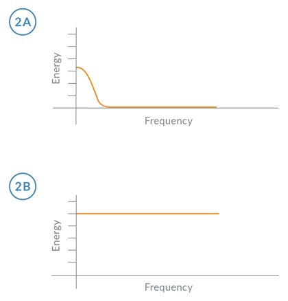
Figure 2: Induced Vibration with an S-Curve Profile and Trapezoidal Profile
How to Minimize Point to Point Transfer Times
Since trapezoidal profiles spend their time at full acceleration or full deceleration, they are, from the standpoint of profile execution, faster than S-curve profiles. But if this 'all on'/'all off' approach causes an increase in settling time, the advantage is lost. Often, only a small amount of "S" (transition between acceleration and no acceleration) can substantially reduce induced vibration. And so to optimize throughput the S-curve profile must be 'tuned' for each a given load and given desired transfer speed.
What S-curve form is right for a given system? On an application by application basis, the specific choice of the form of the S-curve will depend on the mechanical nature of the system, and the desired performance specifications. For example in medical applications which involve liquid transfers that should not be jostled, it would be appropriate to choose a profile with no Phase II & VI segment at all, instead spreading the acceleration transitions out as far as possible, thereby maximizing smoothness.
In other applications involving high speed pick and place, overall transfer speed is most important so a good choice might be an S-curve with transition phases (Phases I, III, V, and VII) that are 5-15 % of Phase II & VI. In this case the S-curve profile will add a small amount of time to the overall transfer time, but because of reduced load oscillation at the end of the move, the total effective transfer time can be considerably decreased. Trial and error using a motion measurement system is generally the best way to determine the right amount of "S", because modelling the response to vibrations is complicated, and not always accurate.
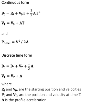
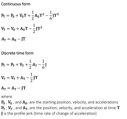
Trapezoidal Trajectory Profile Equations
The basic math required to execute trapezoidal profiles is straightforward. There are, however, two forms that can be used; the continuous form, that will be familiar from High School Physics, and the discrete time form, which is used in most motion systems that utilize microprocessors or DSPs (Digital Signal Processor) to generate a new set of motion parameters at each tick of the motion “clock.”
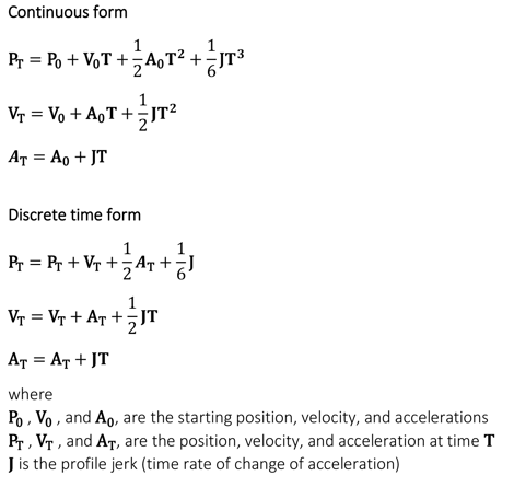
S-Curve Trajectory Profile Equations
Because they are third versus second-order curves, and because there are seven versus three separate motion segments, point-to-point S-curves are more complicated then Trapezoids. In particular it is not simple to calculate the stopping distance for a given set of profile values. Accordingly, many S-curve profiling systems restrict changes-on-the-fly, or do not allow asymmetric profiles. These restrictions allow information about how long, and over what distance, the motion control profile previously took to accelerate to determine when to start decelerating.
Trajectory Profiles for Stepper Motors
The ultimate goal of any profile is to match the motion controller characteristics to the desired application. Trapezoidal and S-curve profiles work well when the motion system's torque response curve is fairly flat. In other words, when the output torque does not vary that much over the range of velocities the system will be experiencing. This is true for most servo motor systems, whether using a brushless motor or a DC Brush motor.
Stepper motors, however, do not have flat torque and speed curves. Torque output is non-linear, sometimes having a large drop at a location called the 'mid-range instability', and generally having drop-off at higher velocities. Figure 3 gives examples of typical torque and speed curves for servo and step-motor systems.
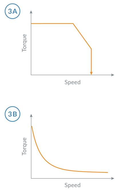
Figure 3: Typical Torque-Speed Curves for Servo Motors and Stepper Motors
Mid-range instability occurs at the step frequency when the motor's natural resonance frequency matches the current step rate. To address mid-range instability, the most common technique is to use a non-zero starting velocity. This means that the profile instantly 'jumps' to a programmed velocity upon initial acceleration, and while decelerating. This is shown in Figure 4. While crude, this technique sometimes provides better results than a smooth ramp for zero, particularly for systems that do not use a microstepping drive technique.
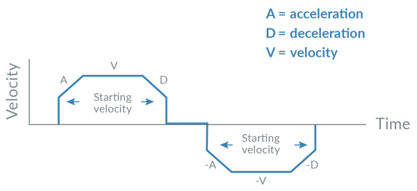
Figure 4: Stepper Motor Profile with Non-Zero Starting Velocity
To address drop-off of torque at higher velocities, a Parabolic profile, shown in Figure 5 can be used. The corresponding acceleration curve has the characteristic that the acceleration is smallest when the velocity is highest. This is a good match for step-motor systems, because there is less torque available at higher speeds. But notice that starting and ending accelerations are very high, and there is no "S" phase where the acceleration smoothly transitions to zero. So if load oscillation is a problem, parabolic profiles may not work as well as an S-curve, despite the fact that a standard S-curve profile is not optimized for a step motor from the standpoint of the torque/speed curve.

Figure 5: Parabolic Trajectory Profile
You may also be interested in: How To Control Stepper Motors
Parabolic Trajectory Profile Equations
Parabolic profiles are closely related to S-curves because they are third-order moves. And as was the case for S-curve profiles, calculating the distance to deceleration is complicated, particularly if profile changes-on-the-fly are allowed.
Stored Motion Profile Tables
The ultimate in point-to-point profile generation, or in fact for other types of profiles including continuous path generation such as is used in CNC (Computer Numerical Control) machine tools, is to construct a custom profile that compensates for the exact load and motor characteristics of the system. Such a profile would accelerate the motor taking into account the available motor torque at each velocity point, the mechanical resonances at each velocity point, and the actuator or arm kinematics in the mechanism.
Since motor torque curves do not follow simple mathematical principles, and because the equations for kinematic compensation are complex, these calculations are generally calculated in advance, and stored in a table of motion 'vectors'. This table is generally set up as an array of position or time vectors, with a corresponding entry for velocity and acceleration at each point of the curve.
It is also possible to include position loop feedforward data in these tables. Normally, the contribution of feedforward terms such as acceleration feedforward to the position loop output can be calculated directly using the profile generator’s acceleration register. But with stored motion profile tables, which break the profile into small segments, this is not possible. To implement a feedforward contribution the desired value is stored as an additional datapoint with each position or velocity table entry and applied to the position loop output as the move is traversed.
With stored motion profiles the motion engine is merely providing a generic capability to download and execute a list of vectors, and the responsibility of the calculations falls to the user. Despite this extra work, if special conditions exist, such as when motors or mechanisms are highly non-linear, table-driven point-to-point profiles can provide a meaningful performance increase and may be worth the effort.
Electronic Cam Profiles
Beyond point-to-point moves, there is a broad range of motion applications that require repetitive motion, indexed by a timer, encoder, or master velocity envelop profile. Such applications fall under the category of electronic cams, which includes the related but simpler approach known as electronic gearing.
Electronic cam profiles typically also use stored motion tables. In this case, the tables are used to define a target position for each location of the encoder or tick of the master clock. The user can download a trapezoidal profile, an S-curve profile, or more commonly, a custom profile that replicates the function of a specially-shaped mechanical cam.
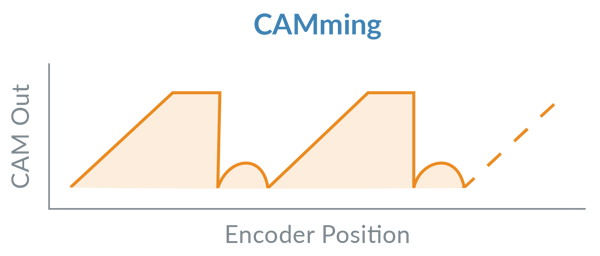
Figure 6: Electronic Cam Profile
There are a number of ways to specify the relationship between the master clock and the controlled axis. The most common is to define the number of encoder counts that make up a 360 degree 'rotation' of the master encoder, and then allow one or more output points to be defined at each degree position of the table. When executing the table, after reading the last location of the table the motion controller will 'wrap' back, and restart from the first. Because of this, the beginning and ending position targets must be the same, or very similar, to avoid a discontinuous jump in motion.
A variation on this approach is to treat each table entry as a relative distance to move rather than as an absolute desired axis location. Using this approach there is no requirement that the first and last entries in the table match up.
Electronic gearing is a simpler version of camming where the relationship between the master can be expressed as a fixed ratio to the driven axis. Gear ratios can be positive or negative, and can be greater or less than one, meaning that the driven axis can amplify, or reduce, the motion specified by the master encoder.
Summary
Choosing the right motion control trajectory profile can improve smoothness, reduce wear, and lower transfer times for a broad range of motion control applications. Trapezoidal trajectory profiles are useful, but limited, because there is no way to define transitions between acceleration regions. S-curve trajectory profiles solve this problem but are correspondingly more complex mathematically. Another important profile for point-to-point trajectory moves is the parabolic profile, generally used only with stepper motor controllers. Stored motion profile table-based approaches to motion profiling are also popular, and in particular, downloadable electronic cams are widely used in a number of industries.
PMD Products with Advanced Profiling Capabilities
PMD has three product groups that provide advanced S-curve and trapezoidal profiles, programmable start velocity, and cam capability. While different in packaging, all are controlled by C-Motion, PMD's easy to use motion control software library and are ideal for use in a wide variety of medical, laboratory, semiconductor, robotic, and industrial motion control applications.

MC58113 Series ICs
The MC58113 series of ICs are part of PMD's popular Magellan Motion Control IC Family and provide advanced position control for stepper, Brushless DC, and DC Brush motors alike. Standard features include FOC (Field Oriented Control), trapezoidal & s-curve profiling, direct encoder and pulse & direction input, and much more. The MC58113 family of ICs are the ideal solution for your next machine design project.
Learn more >>
ION/CME N-Series Drives
ION®/CME N-Series Drives are high performance intelligent drives in an ultra-compact PCB-mountable package. In addition to advanced servo and stepper motor control, N-Series IONs provide S-curve point to point profiling, field oriented control, downloadable user code, general purpose digital and analog I/O, and much more. These all-in-one devices make building your next machine controller a snap.
Learn more >>

Prodigy/CME Machine-Controller
Prodigy®/CME Machine Controller boards provide high-performance motion control for medical, scientific, automation, industrial, and robotic applications. Available in 1, 2, 3, and 4-axis configurations, these boards support DC Brush, Brushless DC, and stepper motors and allow user-written C-language code to be downloaded and run directly on the board. The Prodigy/CME Machine-Controller has on-board Atlas amplifiers that eliminate the need for external amplifiers.
Learn more >>
You may also be interested in:
- How To Optimize Motor Performance Using Motion Trace (Article)
- Field Oriented Control - A Deep Dive(Article)
- S-Curve Motion Profiles - Vital For Optimizing Machine Performance (Article)
- Motion Kinematics (Article)
- How To Control Stepper Motors (Article)