Liquid Handling Robot systems are typically based on a gantry mechanism utilizing X, Y, and Z axis. While fast moves along a single axis can be obtained without undue vibration utilizing S-curve motion profiles, the handling speed is usually a significant factor in determining system throughput; unless other factors prevail, such as a long incubation period and/or a single incubation station. Conventional systems use discrete moves between axes; one axis moves (usually starting with Z) and stops before the next axis is started, resulting in delays when switching directions. Ideally one would utilize an approach wherein a smooth retract in the Z axis is used to clear a well or vial with the pipette tip, and then an automatic transition is made to a coordinated move with all three axes (Z up further to clear obstacles, and X and Y to smoothly transition to the drop-off point) and transition again to the drop-off position (Z-down to get to the well or vial) while still moving in X and Y.
This article (and poster) shows how we have implemented a high-speed motion system on a Liquid Handling Robot gantry that is aware of system clearances so that it can start a planar (X/Y) move while a Z axis move is still ongoing. By employing such a motion control solution, robot move times can be improved by 25% over conventional robot moves and over 50% compared to systems that only employ single axis moves.
Overview
In Liquid Handling Robots that are properly balanced, the gantry robot utilization reaches close to 100%, meaning the robot is almost always moving. In such a situation, improving the move times of the robot can lead to significant throughput enhancements. In systems were (one of) the process steps is a gating factor, the designer should attempt to add parallel process steps to increase throughput. We have measured the move times on a Liquid Handling Robot using a number of different approaches and motion profiles for a robot-limited case. The handling system is able to execute complex moves by injecting a new move profile, while an existing profile is being executed. If the system is aware of clearance heights, it is possible to initiate a move in the X/Y plane while a Z move is ongoing. Further, by employing an S-curve motion profile on all axes, a higher acceleration can be achieved with an equal or better jerk than comparable trapezoidal velocity moves.
The exchange time of the Liquid Handling Robot can be improved by 25%, compared to a system that does not take into account clearances, and by 50% over systems that do not take advantage of combining planar (X/Y) moves.
Liquid Handling Robot (LHR) systems are commonly used for a variety of liquid handling tasks. A significant number of these systems are based on a cartesian gantry system (X, Y and Z axis) and the liquid pump is oftentimes a positive displacement device with a positioning motor (P axis). Although there are many possible process recipes, LHRs are often optimized for a particular set of workflows. In a properly balanced LHR, designed for a certain set of workflows, it is desirable to ensure high throughput, meaning that the gantry itself reaches a utilization of almost 100%. In case a gantry is not 100% utilized, it is sometimes possible to add parallel process stations and thus increase the overall system throughput [1, 2, 3]. In general and for a single end effector, single robot systems, if parallel process stations are used, the throughput is close to optimal if the following relationship is true:
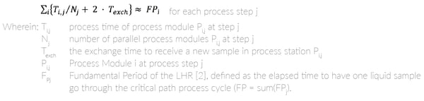
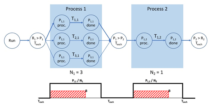
Figure 1: Simple process flow example - Top: Critical path analysis; Bottom: Simplified timing diagram through the critical path.
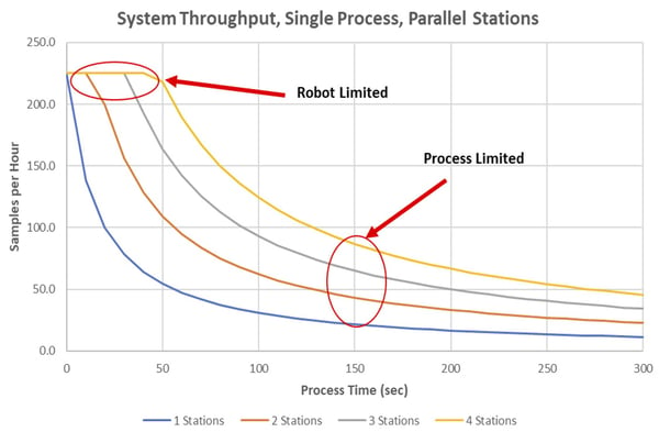
Figure 2: Throughput increase by adding process stations.
There are several simplifying assumptions made in the above equation:
- All process modules P[i,j] have the same process time T[i,j] for all i at step j and behave identically (same process time, no process time variation).
- The sample exchange time T[exch] is essentially the same for any sample transfer, regardless of the distance traveled by the LHR.
- The single robot has a single end effector for liquid transfer, which can be optimized by employing a “pull” strategy for sample handling [3].
- There are no other steps in the flow that cannot be modeled as a “process” step.
In LHR systems where T[i,j] / Nj >> FP/j, for certain steps j, the system throughput will benefit from adding additional process stations Pi,j at the bottleneck process step j. Figure 1, illustrates a simple process flow consisting of a first process running in three parallel process steps and a second process step in a single process station. The critical path (shown in Figure 1, top) shows three transfers and two process steps in series. R[1] > P[1] represents the LHR transfer time from reservoir R[1] to the first set of process stations P[i,1], and conversely P[1] > P[2] represents the transfer from process station P[i,1] to station P[1,2] and P[i,2] > R[2] represents the transfer time from station P[2] to reservoir R[2]. In the present example, there are 8 non-critical path liquid sample transfers; if the 8 transfers take less time than the aggregate process time, the system will not be limited by the LHR, but by the process stations. Therefore three additional equations can be derived:
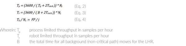
Assuming that the transfer time of the LHR is important in most balanced systems (which in effect means that T[p] = T[r]), it is, therefore, beneficial to increase the system throughput by reducing the average transfer time T[exch]. In more complex systems [4] a detailed decomposition approach may be needed that takes other effects into account such as sample degradation or sample temperature changes during the transfer. For simplicity, those effects are ignored in this paper. Figure 2 models the throughput of Eq 2 and Eq 3 for a single process step with up to four parallel stations. The ideal operating point is at the inflection of the curves when the system throughput is not just limited by the robot transfer time T[exch]. Equation 4 represents that the relative process times (the process times of step j divided by the number of parallel process stations at step j) for each station are equal to each other and to the Fundamental Period FP divided by the number of discrete process steps j.
Methods
Ignoring the one-time effect of the robot coming from a home position to the first reservoir R1, there are generally three ways to move a liquid sample from R1 to a process location P1: each resulting in a different transfer time T[exch]:
- The LHR follows single, individual-axis only moves.
- The LHR follows partially single axis moves, but uses combined moves for the main transfer.
- The LHR uses compound three dimensional moves whenever possible.
Each move can be using a trapezoidal profile, or a more sophisticated S-curve move profile. S-curves are computationally more demanding for the motion system, but can significantly reduce the vibrations injected into the mechanics, allowing for higher overall accelerations with smoother moves. Figure 3 illustrates the three different ways to move a liquid sample.
Mentioned above, each move can be made using a trapezoidal move profile or an S-curve profile. In a trapezoidal move (Figure 4, top), the acceleration is sudden which can result in mechanical vibrations (ringing) in the system as well as in an increase in noise and potential loss of liquid sample. S-curve profiles (Figure 4, bottom) minimize the jerk (derivative of acceleration) during transitions and because this move type results in much less vibration, it allows for faster acceleration after the initial move has started. S-curve profiles can thus take the same or less time than trapezoidal moves.
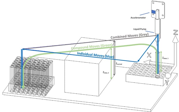
Figure 3: LHR example showing individual (blue), combined (grey), and compound (green) moves.
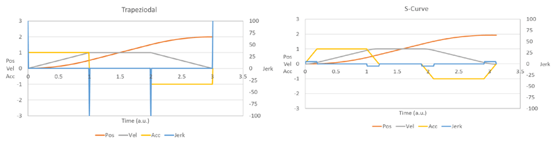
Figure 4: Left: Trapezoidal velocity profile, with high jerk (right axis); Right: S-curve profile.
The complete liquid sample transfer time T[exch] in now decomposed in Figure 5 and Table 1. As seen in Figure 5, bottom, in the conventional move approach there are 10 discrete trapezoidal steps in a single liquid sample transfer cycle T[exch]. Steps 4 and 5 are in the Y and X axis only. Such an approach can be easily improved by making steps 4 and 5 simultaneously, such as is shown in Figure 5, middle. In addition, an S-curve velocity profile can be used for the combined move (dashed line) resulting in a slightly faster T[exch]. Also in Figure 5, top, a compound move approach is shown; a continuous move from the liquid pick-up.
The complete liquid sample transfer time T[exch] in now decomposed in Figure 5 and Table 1. As seen in Figure 5, bottom, in the conventional move approach there are 10 discrete trapezoidal steps in a single liquid sample transfer cycle T[exch]. Steps 4 and 5 are in the Y and X axis only. Such an approach can be easily improved by making steps 4 and 5 simultaneously, such as is shown in Figure 5, middle. In addition, an S-curve velocity profile can be used for the combined move (dashed line) resulting in a slightly faster T[exch].
Also in Figure 5, top, a compound move approach is shown; a continuous move from the liquid pick-up point to the liquid drop-off point, with no stops in-between. The compound move requires awareness of the control system of certain clearance heights in the machine, such as for example those shown in Figure 3: the clearance height of a reagent tube Z[clear], 1, or the clearance height an obstacle Z[clear], 2. The clearance height allows the system to be aware of when it is safe to start an X/Y move. For example, the motion system starts a Z-up move and when the clearance height Z[clear], 1 is reached, the motion system automatically interrupts and switches to an X/Y move, while the Z-move is still active. Similarly, when the system reaches a certain point in the X/Y trajectory, a Z-down move is initiated while the X/Y move is still active, so that the system reaches the clearance height Z[clear], 3 when the X/Y move completes, and then continues in a Z-down only aspect.
By implementing such an interrupt scenario, the T[exch] time can be reduced by some 20%. Depending on the exact process times and number of transfers the LHR has to make, this can represent a significant increase in system throughput. In more complex systems such as those utilizing multiple transfer robots [5, 6], which each robot servicing a number of process stations as well as a number of transfer stations (such as a track system that transfers between LHRs), more handling steps are required in the background process which means that a robot limit can be reached more easily.
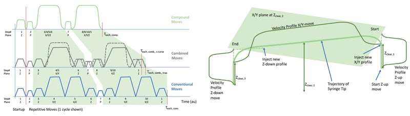
Figure 5: Comparison of conventional moves (bottom), Combined moves (middle), and Compound moves (top).
Figure 6: Timing diagram for Conventional, Combined, and Compound moves.
Results
Table 1 displays the measurements of the individual moves for the conventional, combined and compound moves described above in the background process which means that a robot limit is reached more easily.
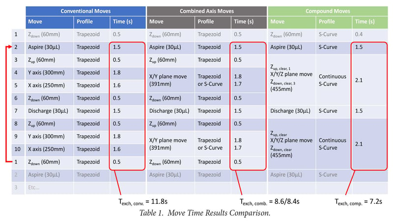
Table 1: Move time results comparison
As seen in Table 1, a conventional moves approach leads to a T[exch] of 11.8s, whereas a combined long move for the X/Y axis reduces that time to 8.6s (8.4 if one uses an S-curve profile). A compound move reduces this further to 7.2s. However, because some of the pump actions are part of the T[exch] time and those are constant, this obscures the improvement a bit. Looking purely at steps 3 through 6, note that the move time went from 4.4s for the conventional to 2.8s for combined moves and to 2.1s for the compound moves. Further improvements are possible by optimizing the higher acceleration using S-curve profiles and properly defined clearances. The improvement will also be larger for longer Z-Moves combined with shorter X/Y moves.
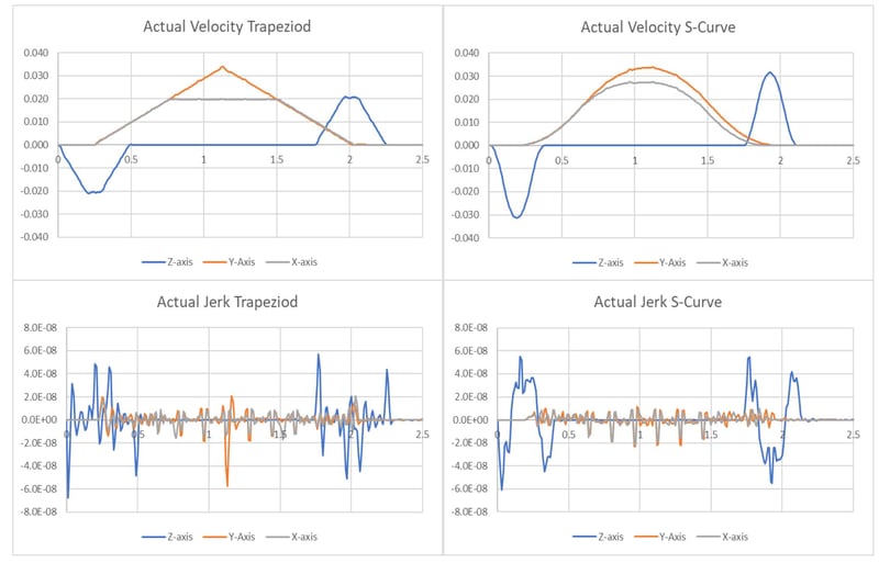
Figure 7: Velocity (top) and jerk (bottom) for trapezoidal (left) and S-curve (right profile moves.
Figure 7 shows the actual velocity for the compound move case using Trapezoidal profiles (left) as well as with S-curve profiles (right) for the same move. As seen in the figure, the S-curve profiles do not have any sudden transitions making them smoother and allowing for higher accelerations and shorter move times, with approximately the same amount of jerk. Furthermore, either case shows that the X/Y moves are started about midway through the Z axis move and similarly for the downward Z move which is initiated when the X and Y axis are still moving. This is a feature of the motion system that was deployed on the gantry in this experiment, allowing real-time injection of a new motion profile while an existing motion profile is still executing.
Conclusion
We have implemented a high-speed motion system on a Liquid Handling Robot gantry that is aware of system clearances so that it can start a planar (X/Y) move while a Z-axis move is still ongoing. The planar move can be initiated after passing a clearance height and by utilizing a trajectory injection method to dynamically change motion trajectories. Similarly, during the arrival near a drop-off point, a Z-axis move can be started while the planar X/Y move is still being executed. By employing such a system, robot move times can be improved by 25% over conventional robot moves and over 50% compared to systems that only employ single axis moves. The use of S-curve motion profiles allows for higher accelerations with a similar or lower jerk as compared to Trapezoidal profile moves.
Acknowledgements
The author thanks Mr. Tom Keller for performing the measurements on the system.
References
[1] M. Pinedo, Scheduling : Theory, Algorithms, and Systems, 2nd ed.
[2] Y. Crama and J. van de Klundert, “Cyclic scheduling of identical parts in a robotic cell,” Oper. Res., vol. 45, no. 6, pp. 952–965, 1997.
[3] M. Dawande, C. Sriskandarajah, and S. Sethi, “On throughput maximization in constant travel-time robotic cells,” Manuf. Service Oper. Manage., vol. 4, no. 4, pp. 296–312, 2002. Upper Saddle River, NJ: Prentice Hall, 2002.
[4] J. Yi, S. Ding, D. Song, and M. T. Zhang, “Steady-State Throughput and Scheduling Analysis of Multi-Cluster Tools: An Decomposition Approach,” IEEE Trans. Autom. Sci. Eng., 2007.
[5] S. Ding, J. Yi, and T.M. Zhang, “Multicluster Tools Scheduling: An Integrated Event Graph and Network Model Approach. IEEE Trans. on Semic. Mfg., vol. 19, no. 3, pp. 339-351, Aug. 2006.
[6] J. Yi, S. Ding, T.M. Zhang and P. van der Meulen, “Throughput Analysis of Linear Cluster Tools”. IEEE Conf. on Autom. Sc. and Eng., pp. 1063-1069., 2007.